EDS 221 Day 8 AM

Factors

---

August 19^th, 2026

Meet the data: gss_cat

---

gss_cat (from forcats) is a sample of the General Social Survey. Several columns store categorical responses.

library(tidyverse)

gss_cat

# A tibble: 21,483 × 9
    year marital         age race  rincome        partyid    relig denom tvhours
   <int> <fct>         <int> <fct> <fct>          <fct>      <fct> <fct>   <int>
 1  2000 Never married    26 White $8000 to 9999  Ind,near … Prot… Sout…      12
 2  2000 Divorced         48 White $8000 to 9999  Not str r… Prot… Bapt…      NA
 3  2000 Widowed          67 White Not applicable Independe… Prot… No d…       2
 4  2000 Never married    39 White Not applicable Ind,near … Orth… Not …       4
 5  2000 Divorced         25 White Not applicable Not str d… None  Not …       1
 6  2000 Married          25 White $20000 - 24999 Strong de… Prot… Sout…      NA
 7  2000 Never married    36 White $25000 or more Not str r… Chri… Not …       3
 8  2000 Divorced         44 White $7000 to 7999  Ind,near … Prot… Luth…      NA
 9  2000 Married          44 White $25000 or more Not str d… Prot… Other       0
10  2000 Married          47 White $25000 or more Strong re… Prot… Sout…       3
# ℹ 21,473 more rows

What is a factor?

---

A factor stores categorical data as a set of predefined levels — the possible values a variable can take.

levels(gss_cat$rincome)

 [1] "No answer"      "Don't know"     "Refused"        "$25000 or more"
 [5] "$20000 - 24999" "$15000 - 19999" "$10000 - 14999" "$8000 to 9999" 
 [9] "$7000 to 7999"  "$6000 to 6999"  "$5000 to 5999"  "$4000 to 4999" 
[13] "$3000 to 3999"  "$1000 to 2999"  "Lt $1000"       "Not applicable"

Under the hood, R stores the values as integers and keeps a lookup table of level labels. This is what makes factors compact and orderable.

Why not just use character strings?

---

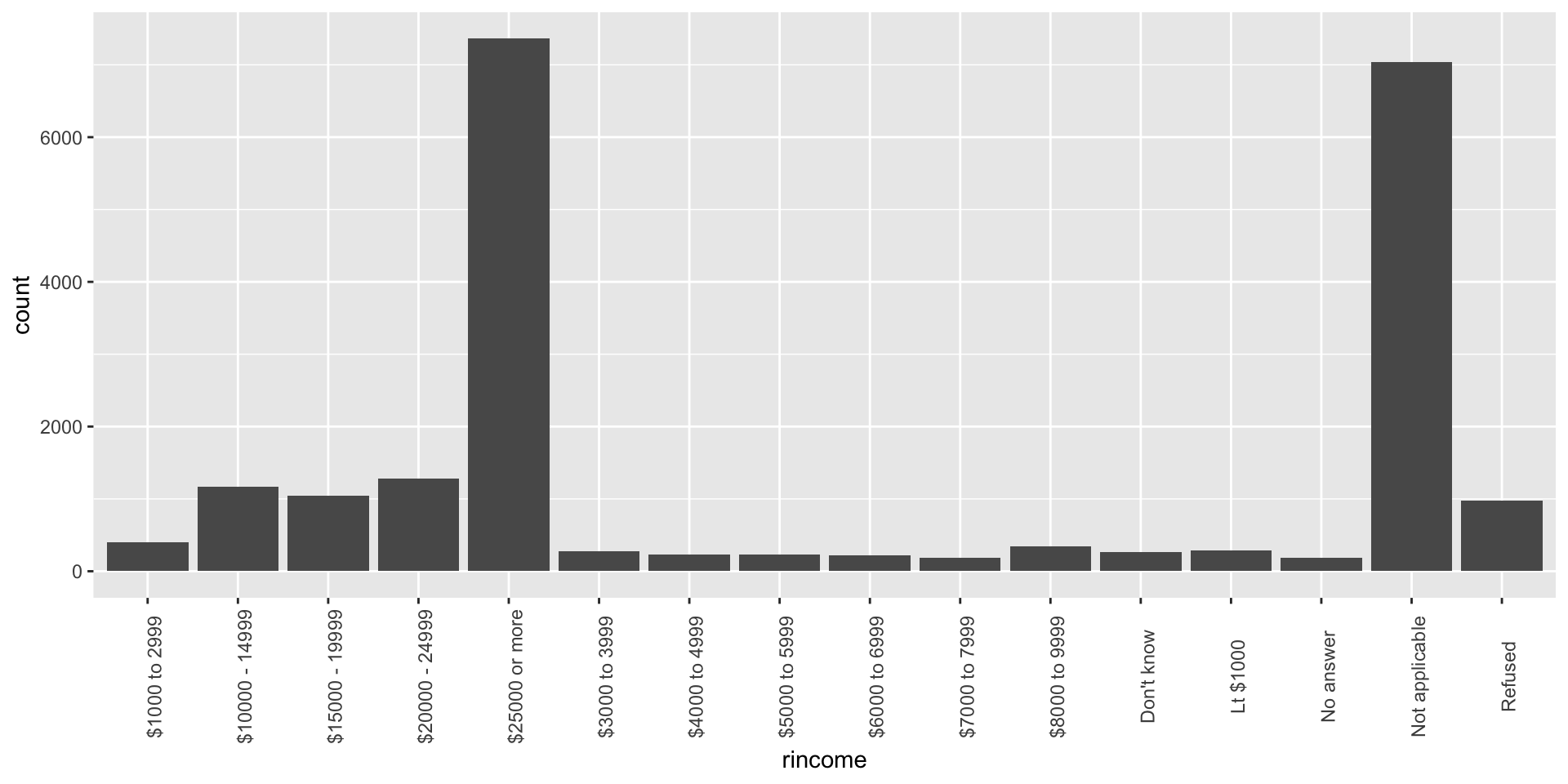
Character vectors sort alphabetically. Factors let you control the order directly, which matters for plots and tables.

gss_cat |>
  mutate(rincome = as.character(rincome)) |>
  ggplot(aes(x = rincome)) +
  geom_bar() +
  theme(axis.text.x = element_text(angle = 90))

Notice the income bins are in no meaningful order — alphabetical, not low-to-high.

fct_relevel(): manual order

---

fct_relevel() moves specific levels to the front, in the order you list them.

gss_cat |>
  mutate(marital = fct_relevel(marital, "Never married", "Married")) |>
  pull(marital) |>
  levels()

[1] "Never married" "Married"       "No answer"     "Separated"    
[5] "Divorced"      "Widowed"      

fct_infreq(): order by frequency

---

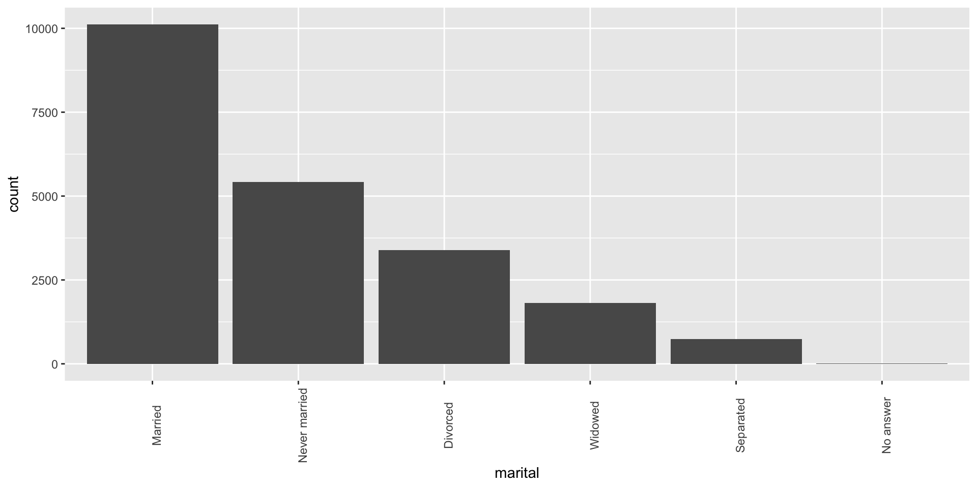
fct_infreq() reorders levels from most to least common — useful whenever “biggest first” is the natural reading order.

gss_cat |>
  mutate(marital = fct_infreq(marital)) |>
  ggplot(aes(x = marital)) +
  geom_bar() +
  theme(axis.text.x = element_text(angle = 90))

fct_reorder(): order by another variable

---

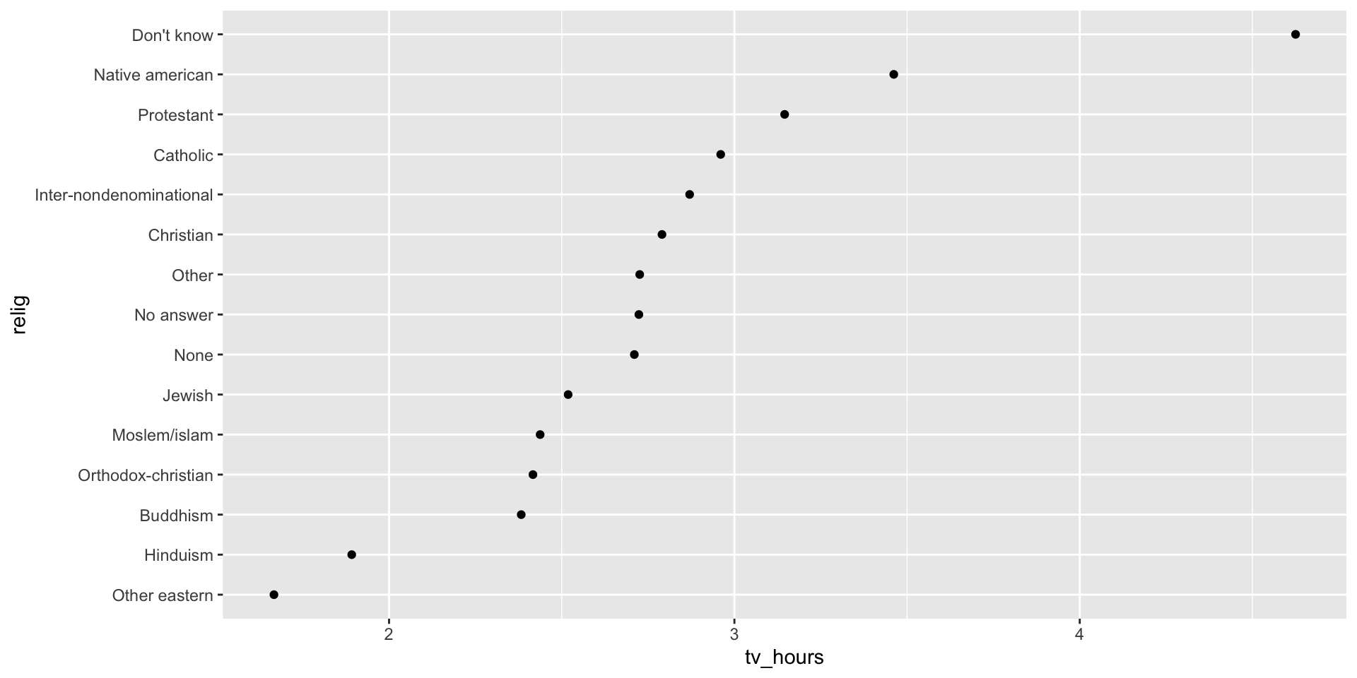
fct_reorder() sorts levels by a summary statistic of another variable — e.g., average TV hours by religion.

relig_summary <- gss_cat |>
  filter(!is.na(tvhours)) |>
  summarize(tv_hours = mean(tvhours), .by = relig)

relig_summary |>
  mutate(relig = fct_reorder(relig, tv_hours)) |>
  ggplot(aes(x = tv_hours, y = relig)) +
  geom_point()

fct_recode(): renaming levels

---

fct_recode() changes level labels without touching the underlying data or order. New name on the left, old name on the right.

gss_cat |>
  mutate(
    partyid = fct_recode(
      partyid,
      "Republican, strong" = "Strong republican",
      "Republican, weak" = "Not str republican"
    )
  ) |>
  count(partyid)

# A tibble: 10 × 2
   partyid                n
   <fct>              <int>
 1 No answer            154
 2 Don't know             1
 3 Other party          393
 4 Republican, strong  2314
 5 Republican, weak    3032
 6 Ind,near rep        1791
 7 Independent         4119
 8 Ind,near dem        2499
 9 Not str democrat    3690
10 Strong democrat     3490

fct_lump(): collapsing rare levels

---

fct_lump_n() keeps the n most common levels and lumps the rest into "Other" — handy when a factor has too many rare categories to plot cleanly.

gss_cat |>
  mutate(relig = fct_lump_n(relig, n = 5)) |>
  count(relig, sort = TRUE)

# A tibble: 6 × 2
  relig          n
  <fct>      <int>
1 Protestant 10846
2 Catholic    5124
3 None        3523
4 Other        913
5 Christian    689
6 Jewish       388

What to memorize

---

Factors store categorical data with explicit, controllable levels instead of relying on alphabetical order.

Inspecting

• levels()

Reordering / recoding

• fct_reorder(), fct_recode()